

Learned emulator: assembling a target shape (JAX / Equinox)#
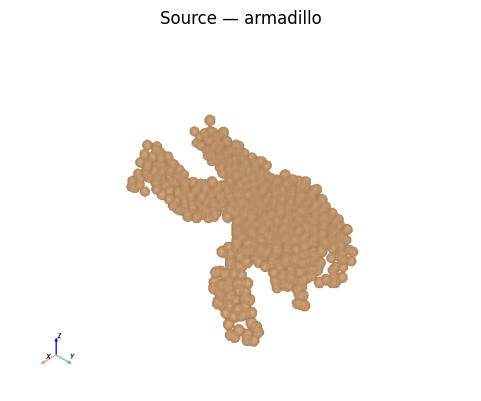
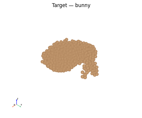
This tutorial trains a Graph Network Simulator (GNS) to assemble one shape into another. Starting from a point cloud sampled on a source mesh (an armadillo), we learn a per-step update rule that deforms it into a target mesh (the Stanford bunny). It is the inverse / learning counterpart to the forward simulator tutorial: instead of hand-specifying mechanochemical rules, we learn them from a shape-matching objective, with gradients flowing through the differentiable Warp physics.
Along the way you will:
sample point clouds from a source and a target mesh,
initialise per-particle state (position, radius, polarity, gene / morphogen channels),
build a contact graph and a GNS that predicts position, polarity and gene updates,
train it end-to-end with an optimal-transport (Sinkhorn) shape loss, and
visualise the learned assembly trajectory.
waxMorph ships this pipeline twice, at parity. This notebook uses the JAX / Equinox backend; the PyTorch version notebook runs the identical workflow on the other backend. Comparing the two is the easiest way to see the differences described in the architecture explanation.
Runtime
This is a deliberately tutorial-scale run (1000 particles, a
50-step rollout, 600 epochs) chosen to finish in a
few minutes on a single GPU. Increase N_POINTS, t_rollout and
n_epochs for a sharper match.
0. Setup#
We quiet XLA’s compile logs and render off-screen so the figures embed as static images.
import os
os.environ.setdefault("TF_CPP_MIN_LOG_LEVEL", "3")  # quiet XLA compile logs

import numpy as np
import matplotlib.pyplot as plt

import pyglet
pyglet.options["headless"] = True
import pyvista as pv
pv.OFF_SCREEN = True

import warp as wp
import jax
import equinox as eqx
import optax

from waxmorph.render import PyVistaInterface

wp.init()
device = "cuda"
np.random.seed(42)
key = jax.random.PRNGKey(42)

# Tutorial-scale configuration.
N_POINTS = 1000
NUM_GENES = 16
T_ROLLOUT = 50
N_EPOCHS = 600
Warp 1.12.1 initialized:
   CUDA Toolkit 12.9, Driver 12.4
   Devices:
     "cpu"      : "x86_64"
     "cuda:0"   : "NVIDIA H100 PCIe" (79 GiB, sm_90, mempool enabled)
   Kernel cache:
     /insomnia001/home/ob2391/.cache/warp/1.12.1
def render_cloud(pos, radii, *, morph=None, polarities=None, title=None,
                 blim=-6.0, tlim=6.0, window_size=(720, 560)):
    """Render a particle cloud to an embedded PNG via an off-screen screenshot.

    We render statically (rather than as an interactive widget) so the figure
    embeds reliably in the built HTML docs.
    """
    n = len(pos)
    if morph is None:
        morph = np.full(n, 0.5, dtype=np.float32)
    if polarities is None:
        polarities = np.zeros((n, 3), dtype=np.float32)
        polarities[:, 2] = 1.0
    plotter = PyVistaInterface.draw_3d_view(
        pos, radii, morph, polarities, particle_count=n,
        blim=blim, tlim=tlim, alpha=0.9, show_polarities=False,
        theta_res=12, phi_res=8,
    )
    plotter.remove_bounds_axes()
    img = plotter.screenshot(return_img=True, window_size=window_size)
    plotter.close()
    fig, ax = plt.subplots(figsize=(window_size[0] / 120, window_size[1] / 120))
    ax.imshow(img)
    ax.axis("off")
    if title:
        ax.set_title(title)
    plt.show()


def render_filmstrip(trajectory, radii, frames, *, blim=-6.0, tlim=6.0,
                     window_size=(360, 320)):
    """Screenshot several rollout frames and lay them out as a filmstrip."""
    shots = []
    n = len(radii)
    morph = np.full(n, 0.5, dtype=np.float32)
    pol = np.zeros((n, 3), dtype=np.float32)
    for f in frames:
        plotter = PyVistaInterface.draw_3d_view(
            trajectory[f], radii, morph, pol, particle_count=n,
            blim=blim, tlim=tlim, alpha=0.9, show_polarities=False,
            theta_res=10, phi_res=6,
        )
        plotter.remove_bounds_axes()
        shots.append((f, plotter.screenshot(return_img=True, window_size=window_size)))
        plotter.close()
    fig, axes = plt.subplots(1, len(shots), figsize=(3.0 * len(shots), 3.0))
    if len(shots) == 1:
        axes = [axes]
    for ax, (f, im) in zip(axes, shots):
        ax.imshow(im)
        ax.axis("off")
        ax.set_title(f"frame {f}")
    fig.suptitle("Learned assembly trajectory (source → target)", y=1.02)
    plt.tight_layout()
    plt.show()
1. Load meshes and sample point clouds#
This is backend-agnostic: sample_mesh_pair
returns NumPy arrays.
from waxmorph.data import sample_mesh_pair

data = sample_mesh_pair(
    source_path="meshes/armadillo.ply",
    target_path="meshes/bunny.ply",
    n_points=N_POINTS,
    source_extent=14.29,
    target_extent=10.0,
)
print(f"source {data['source_pos'].shape}  target {data['target_pos'].shape}")
print(f"source radius {data['source_radius']:.4f}  "
      f"target radius {data['target_radius']:.4f}")
source (1000, 3)  target (1000, 3)
source radius 0.3630  target radius 0.3631
2. Initialise per-particle state#
Identical to the PyTorch notebook: position, radius, unit polarity and gene channels. See the cell-state explanation.
N = len(data["source_pos"])
pos_np = data["source_pos"].copy()
rad_np = np.full(N, data["source_radius"], dtype=np.float32)

rng = np.random.default_rng(42)
pol_np = rng.standard_normal((N, 3)).astype(np.float32)
pol_np /= np.linalg.norm(pol_np, axis=-1, keepdims=True) + 1e-9
genes_np = rng.random((N, NUM_GENES)).astype(np.float32)

print(f"{N} particles, {NUM_GENES} gene channels")
1000 particles, 16 gene channels
Source and target#
render_cloud(data["source_pos"], rad_np, title="Source — armadillo")
target_rad = np.full(len(data["target_pos"]), data["target_radius"], dtype=np.float32)
render_cloud(data["target_pos"], target_rad, title="Target — bunny")
3. Build the GNS#
The JAX build_graph returns a
four-tuple. The extra num_edges is the count of real edges inside a
fixed-size, padded edge buffer (static shapes are what let JAX compile the
rollout). The GNS is an Equinox module, so
it takes an explicit PRNG key and the same dX / dP / dc heads.
from waxmorph.jax.graph import build_graph
from waxmorph.jax.gnn import GNS
from waxmorph.jax.losses import make_sinkhorn_loss

X_probe = wp.from_numpy(pos_np.copy(), dtype=wp.vec3f, device=device)
P_probe = wp.from_numpy(pol_np.copy(), dtype=wp.vec3f, device=device)
R_probe = wp.from_numpy(rad_np.copy(), dtype=wp.float32, device=device)
G_probe = wp.from_numpy(genes_np.copy(), dtype=wp.float32, device=device)

node_feats, edge_index, edge_feats, num_edges = build_graph(
    X_probe, P_probe, R_probe, particle_count=N, c=G_probe,
)
print(f"node features {node_feats.shape}")
print(f"edge index {edge_index.shape}  ({int(num_edges)} real directed edges)")
print(f"edge features {edge_feats.shape}")

model = GNS(
    node_feature_dim=int(node_feats.shape[1]),
    edge_feature_dim=int(edge_feats.shape[1]),
    node_latent_dim=256,
    edge_latent_dim=256,
    hidden_dim=256,
    num_mp_steps=5,
    num_mlp_layers=3,
    output_dims={"dX": 3, "dP": 3, "dc": NUM_GENES},
    checkpoint_processor=True,
    key=key,
)

n_params = sum(x.size for x in jax.tree_util.tree_leaves(eqx.filter(model, eqx.is_array)))
print(f"GNS parameters: {n_params:,}")
node features (1000, 16)
edge index (2, 4212)  (4212 real directed edges)
edge features (4212, 2)
GNS parameters: 3,631,638
The JAX shape loss is the debiased Sinkhorn divergence from ott-jax
(make_sinkhorn_loss; see
the losses explanation). Unlike
PyTorch, Optax optimisers are stateless, so we hold the optimiser state
(opt_state) explicitly and pass it to train.
Loss scale differs across backends
The PyTorch (geomloss) and JAX (ott-jax) Sinkhorn implementations use
different internal scalings, so the absolute loss values are not directly
comparable between the two notebooks. The optimisation behaviour is what
matches: a clearly decreasing curve and a recognisable assembled shape.
loss_fn = make_sinkhorn_loss(blur=0.05)
optimizer = optax.adamw(1e-3)
opt_state = optimizer.init(eqx.filter(model, eqx.is_array))
4. Train#
train has the same signature as the
PyTorch version apart from the explicit opt_state. The first epoch pays a
one-time XLA compilation cost; subsequent epochs are fast. As before, targets
supervises the final rollout frame (t_rollout - 1) against the bunny.
from waxmorph.jax.train import train, TrainConfig

config = TrainConfig(n_epochs=N_EPOCHS, t_rollout=T_ROLLOUT)
targets = [(config.t_rollout - 1, data["target_pos"])]

result = train(
    model, optimizer, opt_state, loss_fn,
    source_pos=data["source_pos"],
    polarities=pol_np,
    c=genes_np,
    radii=rad_np,
    targets=targets,
    config=config,
    device=device,
)
model = result.model
Module waxmorph.emulator abba15d load on device 'cuda:0' took 1222.22 ms (compiled)
Module warp.jax_experimental.ffi 98d2031 load on device 'cuda:0' took 59.52 ms (compiled)
Module waxmorph.jax.warp_autograd 3c963a5 load on device 'cuda:0' took 60.01 ms (compiled)
Epoch 10/600 best=6.2761 shape=6.1696 l2=106.4535
Epoch 20/600 best=5.9285 shape=5.8045 l2=124.0334
Epoch 30/600 best=5.7705 shape=5.6278 l2=142.7044
Epoch 40/600 best=5.6383 shape=5.5001 l2=138.1764
Epoch 50/600 best=5.0680 shape=4.8917 l2=176.2453
Epoch 60/600 best=4.7432 shape=4.5302 l2=212.9556
Epoch 70/600 best=4.7432 shape=4.5302 l2=212.9556
Epoch 80/600 best=4.4862 shape=4.3518 l2=134.3463
Epoch 90/600 best=3.6721 shape=3.4577 l2=214.3992
Epoch 100/600 best=2.8878 shape=2.6227 l2=265.1009
Epoch 110/600 best=2.5414 shape=2.2467 l2=294.6776
Epoch 120/600 best=1.8577 shape=1.6002 l2=257.5338
Epoch 130/600 best=1.5650 shape=1.2756 l2=289.4294
Epoch 140/600 best=1.5650 shape=1.2756 l2=289.4294
Epoch 150/600 best=1.5650 shape=1.2756 l2=289.4294
Epoch 160/600 best=1.4905 shape=1.2304 l2=260.1658
Epoch 170/600 best=1.4005 shape=1.0899 l2=310.6439
Epoch 180/600 best=1.2240 shape=0.9252 l2=298.8226
Epoch 190/600 best=1.1404 shape=0.8394 l2=300.9136
Epoch 200/600 best=1.1404 shape=0.8394 l2=300.9136
Epoch 210/600 best=1.1404 shape=0.8394 l2=300.9136
Epoch 220/600 best=1.1404 shape=0.8394 l2=300.9136
Epoch 230/600 best=1.1404 shape=0.8394 l2=300.9136
Epoch 240/600 best=1.1404 shape=0.8394 l2=300.9136
Epoch 250/600 best=1.1219 shape=0.8277 l2=294.2080
Epoch 260/600 best=1.0805 shape=0.7969 l2=283.5962
Epoch 270/600 best=1.0805 shape=0.7969 l2=283.5962
Epoch 280/600 best=0.9296 shape=0.6404 l2=289.1314
Epoch 290/600 best=0.8995 shape=0.6166 l2=282.8819
Epoch 300/600 best=0.8995 shape=0.6166 l2=282.8819
Epoch 310/600 best=0.8995 shape=0.6166 l2=282.8819
Epoch 320/600 best=0.8190 shape=0.5367 l2=282.2167
Epoch 330/600 best=0.7815 shape=0.4540 l2=327.5090
Epoch 340/600 best=0.7527 shape=0.4425 l2=310.1928
Epoch 350/600 best=0.7164 shape=0.4021 l2=314.2596
Epoch 360/600 best=0.6907 shape=0.3883 l2=302.3939
Epoch 370/600 best=0.6907 shape=0.3883 l2=302.3939
Epoch 380/600 best=0.6247 shape=0.3058 l2=318.9017
Epoch 390/600 best=0.5976 shape=0.2983 l2=299.3319
Epoch 400/600 best=0.5517 shape=0.2541 l2=297.5656
Epoch 410/600 best=0.5151 shape=0.2053 l2=309.8264
Epoch 420/600 best=0.5151 shape=0.2053 l2=309.8264
Epoch 430/600 best=0.5142 shape=0.2211 l2=293.1651
Epoch 440/600 best=0.4810 shape=0.1877 l2=293.2816
Epoch 450/600 best=0.4663 shape=0.1733 l2=292.9806
Epoch 460/600 best=0.4608 shape=0.1773 l2=283.4616
Epoch 470/600 best=0.4608 shape=0.1773 l2=283.4616
Epoch 480/600 best=0.4599 shape=0.1668 l2=293.1047
Epoch 490/600 best=0.4599 shape=0.1668 l2=293.1047
Epoch 500/600 best=0.4411 shape=0.1516 l2=289.5006
Epoch 510/600 best=0.4411 shape=0.1516 l2=289.5006
Epoch 520/600 best=0.4411 shape=0.1516 l2=289.5006
Epoch 530/600 best=0.4375 shape=0.1368 l2=300.6920
Epoch 540/600 best=0.4178 shape=0.1236 l2=294.1715
Epoch 550/600 best=0.4178 shape=0.1236 l2=294.1715
Epoch 560/600 best=0.4178 shape=0.1236 l2=294.1715
Epoch 570/600 best=0.4071 shape=0.1357 l2=271.4453
Epoch 580/600 best=0.4071 shape=0.1357 l2=271.4453
Epoch 590/600 best=0.4035 shape=0.1088 l2=294.6307
Epoch 600/600 best=0.3930 shape=0.1210 l2=272.0270
5. Loss curves#
fig, axes = plt.subplots(1, 3, figsize=(15, 4))
for ax, key, title in zip(
    axes,
    ["losses_shape", "losses_l2", "losses_total"],
    ["Shape (Sinkhorn)", "L2 regulariser", "Total"],
):
    ax.plot(result.log[key])
    ax.set_xlabel("epoch")
    ax.set_ylabel("loss")
    ax.set_title(f"Armadillo → Bunny — {title}")
    ax.grid(True, alpha=0.3)
plt.tight_layout()
plt.show()

print(f"best total loss {result.log['best_loss']:.4f} at epoch {result.log['best_epoch']}")
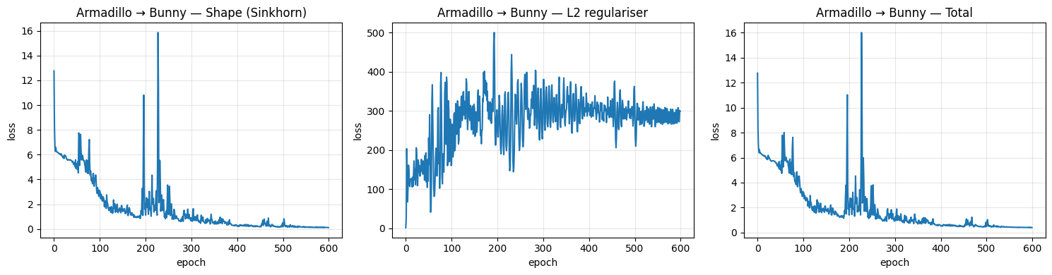
best total loss 0.3930 at epoch 597
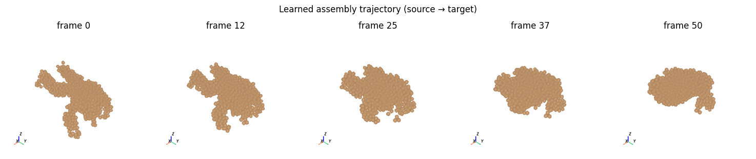
6. The learned assembly#
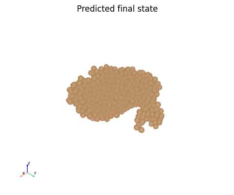
best_traj_pos has shape (t_rollout + 1, N, 3). We render the final frame and
a filmstrip of the trajectory.
trajectory = np.asarray(result.log["best_traj_pos"])
print(f"trajectory {trajectory.shape}, best loss {result.log['best_loss']:.4f}")

render_cloud(trajectory[-1], rad_np, title="Predicted final state")
frames = np.linspace(0, trajectory.shape[0] - 1, 5).astype(int)
render_filmstrip(trajectory, rad_np, frames)
trajectory (51, 1000, 3), best loss 0.3930
7. (Optional) Export a movie#
WarpMovieRenderer is
backend-agnostic and takes NumPy frames.
import os
from waxmorph.render import WarpMovieRenderer

os.makedirs("Output", exist_ok=True)
colors_rgb = np.full((N, 3), [0.3, 0.6, 0.9], dtype=np.float32)

with WarpMovieRenderer(
    filename="Output/armadillo_bunny_jax.usd",
    max_particles=N,
    backend="usd",
    fps=30,
    device=device,
) as mov:
    for f in range(trajectory.shape[0]):
        mov.write_frame_from_numpy(
            t=float(f) / 30.0,
            centers=trajectory[f],
            radii=rad_np,
            colors=colors_rgb,
            particle_count=N,
        )
print("wrote Output/armadillo_bunny_jax.usd")
Saved the USD stage file at `/insomnia001/depts/morpheus/users/ob2391/Waxmorph/Output/armadillo_bunny_jax.usd`
wrote Output/armadillo_bunny_jax.usd