

Learned emulator: assembling a target shape (PyTorch)#
This tutorial trains a Graph Network Simulator (GNS) to assemble one shape into another. Starting from a point cloud sampled on a source mesh (an armadillo), we learn a per-step update rule that deforms it into a target mesh (the Stanford bunny). It is the inverse / learning counterpart to the forward simulator tutorial: instead of hand-specifying mechanochemical rules, we learn them from a shape-matching objective, with gradients flowing through the differentiable Warp physics.
Along the way you will:
sample point clouds from a source and a target mesh,
initialise per-particle state (position, radius, polarity, gene / morphogen channels),
build a contact graph and a GNS that predicts position, polarity and gene updates,
train it end-to-end with an optimal-transport (Sinkhorn) shape loss, and
visualise the learned assembly trajectory.
waxMorph ships this pipeline twice, at parity. This notebook uses the PyTorch backend; the JAX version notebook runs the identical workflow on the other backend. Comparing the two is the easiest way to see the differences described in the architecture explanation.
Runtime
This is a deliberately tutorial-scale run (1000 particles, a
50-step rollout, 600 epochs) chosen to finish in a
few minutes on a single GPU. Increase N_POINTS, t_rollout and
n_epochs for a sharper match.
0. Setup#
We render off-screen (headless) so the figures embed as static images in the docs.
import numpy as np
import matplotlib.pyplot as plt

import pyglet
pyglet.options["headless"] = True
import pyvista as pv
pv.OFF_SCREEN = True

import warp as wp
import torch

from waxmorph.render import PyVistaInterface

wp.init()
device = "cuda"
torch_device = torch.device("cuda")
np.random.seed(42)
torch.manual_seed(42)

# Tutorial-scale configuration.
N_POINTS = 1000
NUM_GENES = 16
T_ROLLOUT = 50
N_EPOCHS = 600
Warp 1.12.1 initialized:
   CUDA Toolkit 12.9, Driver 12.4
   Devices:
     "cpu"      : "x86_64"
     "cuda:0"   : "NVIDIA H100 PCIe" (79 GiB, sm_90, mempool enabled)
   Kernel cache:
     /insomnia001/home/ob2391/.cache/warp/1.12.1
def render_cloud(pos, radii, *, morph=None, polarities=None, title=None,
                 blim=-6.0, tlim=6.0, window_size=(720, 560)):
    """Render a particle cloud to an embedded PNG via an off-screen screenshot.

    We render statically (rather than as an interactive widget) so the figure
    embeds reliably in the built HTML docs.
    """
    n = len(pos)
    if morph is None:
        morph = np.full(n, 0.5, dtype=np.float32)
    if polarities is None:
        polarities = np.zeros((n, 3), dtype=np.float32)
        polarities[:, 2] = 1.0
    plotter = PyVistaInterface.draw_3d_view(
        pos, radii, morph, polarities, particle_count=n,
        blim=blim, tlim=tlim, alpha=0.9, show_polarities=False,
        theta_res=12, phi_res=8,
    )
    plotter.remove_bounds_axes()
    img = plotter.screenshot(return_img=True, window_size=window_size)
    plotter.close()
    fig, ax = plt.subplots(figsize=(window_size[0] / 120, window_size[1] / 120))
    ax.imshow(img)
    ax.axis("off")
    if title:
        ax.set_title(title)
    plt.show()


def render_filmstrip(trajectory, radii, frames, *, blim=-6.0, tlim=6.0,
                     window_size=(360, 320)):
    """Screenshot several rollout frames and lay them out as a filmstrip."""
    shots = []
    n = len(radii)
    morph = np.full(n, 0.5, dtype=np.float32)
    pol = np.zeros((n, 3), dtype=np.float32)
    for f in frames:
        plotter = PyVistaInterface.draw_3d_view(
            trajectory[f], radii, morph, pol, particle_count=n,
            blim=blim, tlim=tlim, alpha=0.9, show_polarities=False,
            theta_res=10, phi_res=6,
        )
        plotter.remove_bounds_axes()
        shots.append((f, plotter.screenshot(return_img=True, window_size=window_size)))
        plotter.close()
    fig, axes = plt.subplots(1, len(shots), figsize=(3.0 * len(shots), 3.0))
    if len(shots) == 1:
        axes = [axes]
    for ax, (f, im) in zip(axes, shots):
        ax.imshow(im)
        ax.axis("off")
        ax.set_title(f"frame {f}")
    fig.suptitle("Learned assembly trajectory (source → target)", y=1.02)
    plt.tight_layout()
    plt.show()
1. Load meshes and sample point clouds#
sample_mesh_pair loads two meshes,
recentres and rescales them to a common world size, and samples a point cloud
from each surface. source_extent / target_extent set the bounding-box size
each mesh is normalised to, which also fixes a sphere radius per particle.
from waxmorph.data import sample_mesh_pair

data = sample_mesh_pair(
    source_path="meshes/armadillo.ply",
    target_path="meshes/bunny.ply",
    n_points=N_POINTS,
    source_extent=14.29,
    target_extent=10.0,
)
print(f"source {data['source_pos'].shape}  target {data['target_pos'].shape}")
print(f"source radius {data['source_radius']:.4f}  "
      f"target radius {data['target_radius']:.4f}")
source (1000, 3)  target (1000, 3)
source radius 0.3630  target radius 0.3631
2. Initialise per-particle state#
Each cell-like agent carries a position, a radius, a unit polarity vector, and a vector of gene / morphogen channels. We start the positions on the source mesh; polarities are random unit vectors and genes are random (the GNS will learn to drive them). See the cell-state explanation for what each field means.
N = len(data["source_pos"])
pos_np = data["source_pos"].copy()
rad_np = np.full(N, data["source_radius"], dtype=np.float32)

rng = np.random.default_rng(42)
pol_np = rng.standard_normal((N, 3)).astype(np.float32)
pol_np /= np.linalg.norm(pol_np, axis=-1, keepdims=True) + 1e-9
genes_np = rng.random((N, NUM_GENES)).astype(np.float32)

print(f"{N} particles, {NUM_GENES} gene channels")
1000 particles, 16 gene channels
Source and target#
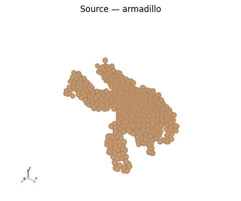
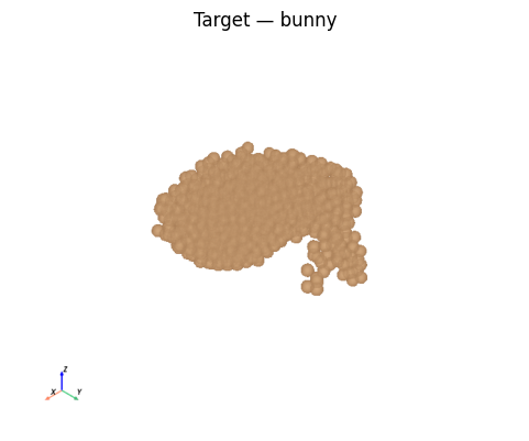
The learned emulator must deform the source cloud (left) into the target cloud (right).
render_cloud(data["source_pos"], rad_np, title="Source — armadillo")
target_rad = np.full(len(data["target_pos"]), data["target_radius"], dtype=np.float32)
render_cloud(data["target_pos"], target_rad, title="Target — bunny")
3. Build the GNS#
build_graph turns the
current state into a contact graph: node
features per particle and edge features per contact. We probe it once to size the
network. The GNS has three output heads: dX
(position update), dP (polarity update) and dc (gene update). Its
gradients flow back through the Warp physics during the rollout.
from waxmorph.graph import build_graph
from waxmorph.gnn import GNS
from waxmorph.losses import make_samples_loss

X_probe = wp.from_numpy(pos_np.copy(), dtype=wp.vec3f, device=device)
P_probe = wp.from_numpy(pol_np.copy(), dtype=wp.vec3f, device=device)
R_probe = wp.from_numpy(rad_np.copy(), dtype=wp.float32, device=device)
G_probe = wp.from_numpy(genes_np.copy(), dtype=wp.float32, device=device)

node_feats, edge_index, edge_feats = build_graph(
    X_probe, P_probe, R_probe, particle_count=N, c=G_probe,
)
print(f"node features {node_feats.shape}")
print(f"edge index {edge_index.shape}  ({edge_index.shape[1]} directed edges)")
print(f"edge features {edge_feats.shape}")

model = GNS(
    node_feature_dim=node_feats.shape[1],
    edge_feature_dim=edge_feats.shape[1],
    node_latent_dim=256,
    edge_latent_dim=256,
    hidden_dim=256,
    num_mp_steps=5,
    num_mlp_layers=3,
    output_dims={"dX": 3, "dP": 3, "dc": NUM_GENES},
    checkpoint_processor=True,
).to(torch_device)

n_params = sum(p.numel() for p in model.parameters())
print(f"GNS parameters: {n_params:,}")
node features torch.Size([1000, 16])
edge index torch.Size([2, 4212])  (4212 directed edges)
edge features torch.Size([4212, 2])
GNS parameters: 3,631,638
The shape loss compares the predicted and target clouds as unordered point
sets. We use the debiased Sinkhorn divergence (an entropic optimal-transport
approximation of the 2-Wasserstein distance) via
make_samples_loss; see
the losses explanation. On PyTorch the optimiser state
lives inside the torch.optim object.
loss_fn = make_samples_loss(loss="sinkhorn", blur=0.05)
optimizer = torch.optim.AdamW(model.parameters(), lr=1e-3)
[KeOps] Compiling cuda jit compiler engine ...
OK
[pyKeOps] Compiling nvrtc binder for python ...
OK
4. Train#
train runs the differentiable
rollout: from the source state it applies t_rollout GNS updates (each followed
by the Warp mechanics/diffusion sub-steps), compares the result against the
supervision targets, and backpropagates. targets is a list of
(frame_index, target_cloud) pairs; here we supervise the final rollout
frame (t_rollout - 1) against the bunny.
With 1000 particles and a 50-step rollout this takes a few minutes per 600-epoch run on one GPU.
from waxmorph.train import train, TrainConfig

config = TrainConfig(n_epochs=N_EPOCHS, t_rollout=T_ROLLOUT)
targets = [(config.t_rollout - 1, data["target_pos"])]

result = train(
    model, optimizer, loss_fn,
    source_pos=data["source_pos"],
    polarities=pol_np,
    c=genes_np,
    radii=rad_np,
    targets=targets,
    config=config,
    device=device,
)
model = result.model
Module waxmorph.emulator abba15d load on device 'cuda:0' took 1056.18 ms (compiled)
Epoch 10/600 best=2.9606 shape=2.8617 l2=98.8823
Epoch 20/600 best=2.9442 shape=2.8179 l2=126.3093
Epoch 30/600 best=2.7840 shape=2.6487 l2=135.3209
Epoch 40/600 best=2.7101 shape=2.5671 l2=143.0124
Epoch 50/600 best=2.5841 shape=2.4161 l2=167.9542
Epoch 60/600 best=2.3649 shape=2.1935 l2=171.4096
Epoch 70/600 best=1.9745 shape=1.7435 l2=231.0038
Epoch 80/600 best=1.2689 shape=0.9329 l2=335.9413
Epoch 90/600 best=0.8686 shape=0.5417 l2=326.8400
Epoch 100/600 best=0.7764 shape=0.4489 l2=327.5516
Epoch 110/600 best=0.7764 shape=0.4489 l2=327.5516
Epoch 120/600 best=0.7764 shape=0.4489 l2=327.5516
Epoch 130/600 best=0.7403 shape=0.4653 l2=274.9466
Epoch 140/600 best=0.7318 shape=0.4369 l2=294.9376
Epoch 150/600 best=0.6475 shape=0.3600 l2=287.4379
Epoch 160/600 best=0.6385 shape=0.3543 l2=284.2050
Epoch 170/600 best=0.6134 shape=0.3135 l2=299.9210
Epoch 180/600 best=0.5707 shape=0.2808 l2=289.8889
Epoch 190/600 best=0.5515 shape=0.2771 l2=274.3623
Epoch 200/600 best=0.5457 shape=0.2202 l2=325.5191
Epoch 210/600 best=0.5317 shape=0.2560 l2=275.7029
Epoch 220/600 best=0.4817 shape=0.1779 l2=303.7665
Epoch 230/600 best=0.4817 shape=0.1779 l2=303.7665
Epoch 240/600 best=0.4817 shape=0.1779 l2=303.7665
Epoch 250/600 best=0.4817 shape=0.1779 l2=303.7665
Epoch 260/600 best=0.4555 shape=0.2021 l2=253.3754
Epoch 270/600 best=0.4052 shape=0.1240 l2=281.1507
Epoch 280/600 best=0.4024 shape=0.1185 l2=283.9742
Epoch 290/600 best=0.4024 shape=0.1185 l2=283.9742
Epoch 300/600 best=0.3910 shape=0.1095 l2=281.4763
Epoch 310/600 best=0.3786 shape=0.0882 l2=290.4792
Epoch 320/600 best=0.3762 shape=0.1122 l2=264.0439
Epoch 330/600 best=0.3762 shape=0.1122 l2=264.0439
Epoch 340/600 best=0.3755 shape=0.0994 l2=276.0947
Epoch 350/600 best=0.3673 shape=0.1102 l2=257.0679
Epoch 360/600 best=0.3673 shape=0.1102 l2=257.0679
Epoch 370/600 best=0.3655 shape=0.0960 l2=269.5772
Epoch 380/600 best=0.3655 shape=0.0960 l2=269.5772
Epoch 390/600 best=0.3519 shape=0.0770 l2=274.8630
Epoch 400/600 best=0.3475 shape=0.0884 l2=259.0420
Epoch 410/600 best=0.3434 shape=0.0722 l2=271.2558
Epoch 420/600 best=0.3434 shape=0.0722 l2=271.2558
Epoch 430/600 best=0.3434 shape=0.0722 l2=271.2558
Epoch 440/600 best=0.3434 shape=0.0722 l2=271.2558
Epoch 450/600 best=0.3434 shape=0.0722 l2=271.2558
Epoch 460/600 best=0.3396 shape=0.0805 l2=259.1278
Epoch 470/600 best=0.3396 shape=0.0805 l2=259.1278
Epoch 480/600 best=0.3347 shape=0.0640 l2=270.6834
Epoch 490/600 best=0.3306 shape=0.0774 l2=253.2574
Epoch 500/600 best=0.3296 shape=0.0612 l2=268.3848
Epoch 510/600 best=0.3269 shape=0.0587 l2=268.2107
Epoch 520/600 best=0.3248 shape=0.0739 l2=250.8620
Epoch 530/600 best=0.3246 shape=0.0796 l2=245.0643
Epoch 540/600 best=0.3195 shape=0.0613 l2=258.2401
Epoch 550/600 best=0.3176 shape=0.0528 l2=264.7588
Epoch 560/600 best=0.3176 shape=0.0528 l2=264.7588
Epoch 570/600 best=0.3098 shape=0.0509 l2=258.9607
Epoch 580/600 best=0.3054 shape=0.0481 l2=257.3250
Epoch 590/600 best=0.3045 shape=0.0414 l2=263.0889
Epoch 600/600 best=0.3045 shape=0.0414 l2=263.0889
5. Loss curves#
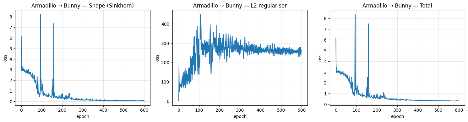
losses_shape is the Sinkhorn shape term, losses_l2 the displacement regulariser, losses_total their weighted sum.
fig, axes = plt.subplots(1, 3, figsize=(15, 4))
for ax, key, title in zip(
    axes,
    ["losses_shape", "losses_l2", "losses_total"],
    ["Shape (Sinkhorn)", "L2 regulariser", "Total"],
):
    ax.plot(result.log[key])
    ax.set_xlabel("epoch")
    ax.set_ylabel("loss")
    ax.set_title(f"Armadillo → Bunny — {title}")
    ax.grid(True, alpha=0.3)
plt.tight_layout()
plt.show()

print(f"best total loss {result.log['best_loss']:.4f} at epoch {result.log['best_epoch']}")
best total loss 0.3045 at epoch 585
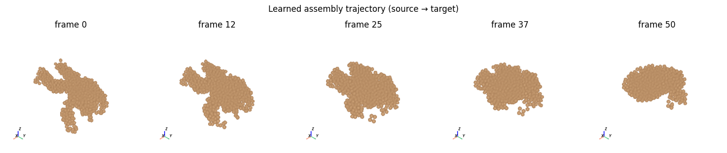
6. The learned assembly#
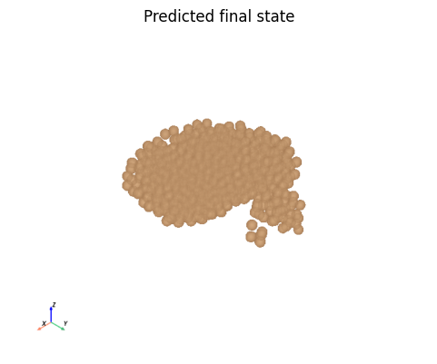
train records the best-scoring rollout. best_traj_pos has shape
(t_rollout + 1, N, 3): the source cloud followed by every updated frame.
We render the final frame and a filmstrip of the full trajectory.
trajectory = result.log["best_traj_pos"]
print(f"trajectory {trajectory.shape}, best loss {result.log['best_loss']:.4f}")

render_cloud(trajectory[-1], rad_np, title="Predicted final state")
frames = np.linspace(0, trajectory.shape[0] - 1, 5).astype(int)
render_filmstrip(trajectory, rad_np, frames)
trajectory (51, 1000, 3), best loss 0.3045
7. (Optional) Export a movie#
WarpMovieRenderer writes the
trajectory to a USD stage (for Blender / usdview) or, with backend="opengl",
to an MP4. This produces a file rather than an inline figure.
import os
from waxmorph.render import WarpMovieRenderer

os.makedirs("Output", exist_ok=True)
colors_rgb = np.full((N, 3), [0.3, 0.6, 0.9], dtype=np.float32)

with WarpMovieRenderer(
    filename="Output/armadillo_bunny.usd",
    max_particles=N,
    backend="usd",
    fps=30,
    device=device,
) as mov:
    for f in range(trajectory.shape[0]):
        mov.write_frame_from_numpy(
            t=float(f) / 30.0,
            centers=trajectory[f],
            radii=rad_np,
            colors=colors_rgb,
            particle_count=N,
        )
print("wrote Output/armadillo_bunny.usd")
Saved the USD stage file at `/insomnia001/depts/morpheus/users/ob2391/Waxmorph/Output/armadillo_bunny.usd`
wrote Output/armadillo_bunny.usd